Chapter 4 (Vector Spaces): Coordinate systems (坐标系)
本文共 5352 字,大约阅读时间需要 17 分钟。
本文为《Linear algebra and its applications》的读书笔记
目录
Coordinate systems
- An important reason for specifying a basis B \mathcal B B for a vector space V V V is to impose a “coordinate system” on V V V .
- This section will show that if B \mathcal B B contains n n n vectors, then the coordinate system will make V V V act like R n \mathbb R^n Rn. If V V V is already R n \mathbb R^n Rn itself, then B \mathcal B B will determine a coordinate system that gives a new “view” of V V V .
- The existence of coordinate systems rests on the following fundamental result.

- Since B \mathcal B B spans V V V, there exist scalars such that (1) holds. Suppose x \boldsymbol x x also has the representation
 Then, subtracting, we have
  Since B \mathcal B B is linearly independent, the weights must all be zero. That is, c j = d j c_j = d_j cj=dj for 1 ≤ j ≤ n 1 \leq j \leq n 1≤j≤n.
Be careful not to use a matrix in the proof. The vectors v 1 , . . . , v n \boldsymbol v_1,..., \boldsymbol v_n v1,...,vn cannot be arranged as the columns of an ordinary matrix when the vectors are in some abstract vector space.
- If c 1 , . . . , c n c_1,..., c_n c1,...,cn are the B \mathcal B B-coordinates of x \boldsymbol x x, then the vector in R n \mathbb R^n Rn
 is the coordinate vector of x \boldsymbol x x (relative to B \mathcal B B, or the B \mathcal B B-coordinate vector of x \boldsymbol x x). The mapping x ↦ [ x ] B \boldsymbol x \mapsto [\boldsymbol x]_{\mathcal B} x↦[x]B is the coordinate mapping (determined by B \mathcal B B).
A Graphical Interpretation of Coordinates
- A coordinate system on a set consists of a one-to-one mapping of the points in the set into R n \mathbb R^n Rn.
- For example, ordinary graph paper provides a coordinate system for the plane when one selects perpendicular axes and a unit of measurement on each axis. Figure 1 shows the vector x = [ 1 6 ] \boldsymbol x=\begin{bmatrix}1\\6\end{bmatrix} x=[16]. The coordinates 1 and 6 give the location of x \boldsymbol x x relative to the standard basis { e 1 , e 2 } \{\boldsymbol e_1, \boldsymbol e_2\} { e1,e2}: 1 unit in the e 1 \boldsymbol e_1 e1 direction and 6 units in the e2 direction.
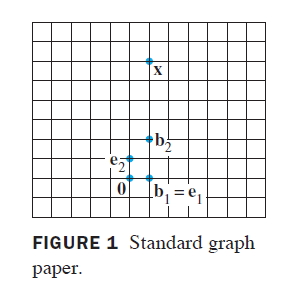
- Figure 2 shows the vector x \boldsymbol x x from Figure 1. However, the standard coordinate grid was erased and replaced by a grid especially adapted to the basis B = { [ 1 0 ] , [ 1 2 ] } \mathcal B=\{\begin{bmatrix}1\\0\end{bmatrix},\begin{bmatrix}1\\2\end{bmatrix}\} B={ [10],[12]}. The coordinate vector [ x ] B = [ − 2 3 ] [\boldsymbol x]_{\mathcal B}=\begin{bmatrix}-2\\3\end{bmatrix} [x]B=[−23] gives the location of x \boldsymbol x x on this new coordinate system: -2 units in the b 1 \boldsymbol b_1 b1 direction and 3 units in the b 2 \boldsymbol b_2 b2 direction.

- For example, ordinary graph paper provides a coordinate system for the plane when one selects perpendicular axes and a unit of measurement on each axis. Figure 1 shows the vector x = [ 1 6 ] \boldsymbol x=\begin{bmatrix}1\\6\end{bmatrix} x=[16]. The coordinates 1 and 6 give the location of x \boldsymbol x x relative to the standard basis { e 1 , e 2 } \{\boldsymbol e_1, \boldsymbol e_2\} { e1,e2}: 1 unit in the e 1 \boldsymbol e_1 e1 direction and 6 units in the e2 direction.
Coordinates in R n \mathbb R^n Rn
- When a basis B \mathcal B B for R n \mathbb R^n Rn is fixed, the B \mathcal B B-coordinate vector of a specified x \boldsymbol x x is easily found.
- Let
 Then the vector equation
  is equivalent to
- We call P B P_B PB the change-of-coordinates matrix (坐标变换矩阵) from B \mathcal B B to the standard basis in R n \mathbb R^n Rn.
- Left-multiplication by P B P_B PB transforms the coordinate vector [ x ] B [\boldsymbol x]_{\mathcal B} [x]B into x \boldsymbol x x.
- Since the columns of P B P_B PB form a basis for R n \mathbb R^n Rn, P B P_B PB is invertible. Left-multiplication by P B − 1 P_B^{-1} PB−1 converts x \boldsymbol x x into its B \mathcal B B-coordinate vector:
 The correspondence x ↦ [ x ] B \boldsymbol x\mapsto [\boldsymbol x]_{\mathcal B} x↦[x]B, produced here by P B − 1 P_B^{-1} PB−1, is the coordinate mapping mentioned earlier. Since P B − 1 P_B^{-1} PB−1 is an invertible matrix, the coordinate mapping is a one-to-one linear transformation from R n \mathbb R^n Rn onto R n \mathbb R^n Rn. This property of the coordinate mapping is also true in a general vector space that has a basis.
The Coordinate Mapping
- Choosing a basis B = { b 1 , . . . , b n } \mathcal B = \{\boldsymbol b_1,..., \boldsymbol b_n\} B={ b1,...,bn} for a vector space V V V introduces a coordinate system in V V V . The coordinate mapping x ↦ [ x ] B \boldsymbol x\mapsto [\boldsymbol x]_{\mathcal B} x↦[x]B connects the possibly unfamiliar space V V V to the familiar space R n \mathbb R^n Rn. See Figure 5.

- Take two typical vectors in V V V , say,
 Then, using vector operations,
  It follows that
  If r r r is any scalar, then
  So
So  Thus the coordinate mapping is a linear transformation. It is easy to show that the coordinate mapping is one-to-one and maps V V V onto R n \mathbb R^n Rn.
- The linearity of the coordinate mapping extends to linear combination:
 The coordinate mapping in Theorem 8 is an important example of an isomorphism (同构) from V V V onto R n \mathbb R^n Rn.
 - In particular, any real vector space with a basis of n n n vectors is indistinguishable from R n \mathbb R^n Rn.

EXAMPLE 5
- Let B \mathcal B B be the standard basis of the space P 3 \mathbb P^3 P3 of polynomials; that is, let B = { 1 , t , t 2 , t 3 } \mathcal B =\{1, t, t^2, t^3\} B={ 1,t,t2,t3}. A typical element p \boldsymbol p p of P 3 \mathbb P^3 P3 has the form
 Thus the coordinate mapping p ↦ [ p ] B \boldsymbol p \mapsto [\boldsymbol p]_{\mathcal B} p↦[p]B is an isomorphism from P 3 \mathbb P^3 P3 onto R 4 \mathbb R^4 R4. All vector space operations in P 3 \mathbb P^3 P3 correspond to operations in R 4 \mathbb R^4 R4.
转载地址:http://clih.baihongyu.com/
你可能感兴趣的文章
Netty工作笔记0084---通过自定义协议解决粘包拆包问题2
查看>>
Netty工作笔记0085---TCP粘包拆包内容梳理
查看>>
Netty常用组件一
查看>>
Netty常见组件二
查看>>
Netty应用实例
查看>>
netty底层——nio知识点 ByteBuffer+Channel+Selector
查看>>
netty底层源码探究:启动流程;EventLoop中的selector、线程、任务队列;监听处理accept、read事件流程;
查看>>
Netty心跳检测
查看>>
Netty心跳检测机制
查看>>
netty既做服务端又做客户端_网易新闻客户端广告怎么做
查看>>
netty时间轮
查看>>
Netty服务端option配置SO_REUSEADDR
查看>>
Netty核心模块组件
查看>>
Netty框架内的宝藏:ByteBuf
查看>>
Netty框架的服务端开发中创建EventLoopGroup对象时线程数量源码解析
查看>>
Netty源码—1.服务端启动流程一
查看>>
Netty源码—1.服务端启动流程二
查看>>
Netty源码—2.Reactor线程模型一
查看>>
Netty源码—2.Reactor线程模型二
查看>>
Netty源码—3.Reactor线程模型三
查看>>